Exit velocity is an important metric coming from Statcast data. However, all too often public analyses use “average exit velocity,” and much is lost in doing so. When looking at various outcome metrics like slugging percentage or wOBA, there is practically no difference between a batted ball with an exit velocity of 65 MPH and one with 75 MPH. However, there is a huge difference between 95 and 105 for instance. If player A hits one ball at 110 , another at 115, and a third at 30 MPH, he has an average exit velocity of 85. If player B hits three balls at 84, 85, and 86 MPH, he has the same average of 85. However, player A will likely have much better outcomes than player B; two rockets and a dribbler are probably better than three mediocre balls in play that are each likely to be outs.

Because of this nonlinear nature between productivity and exit velocity, I think looking at the entire distribution of a player’s exit velocity is important, rather than just the mean. In order to use this information for other analyses (for instance as a prior in my CASSIE projections), I wanted to parameterize this distribution. Other techniques like histograms or kernel density estimations do allow us to visualize the distribution, but a simple parameterization can prove helpful for more in-depth analysis than simply visualization.

In viewing histograms of the exit velocity for a variety of players, I hypothesized that they could be well-characterized as a mixture of two normal distributions (thus producing two peaks). One peak would be centered around well-struck, “barrelled” balls, while the other peak would be centered around more weakly contacted balls. Whereas a normal distribution is characterized by its mean and standard deviation, this mixture of two normals is characterized by two means, two standard deviations, and a mixing parameter that measures how often to draw from one distribution vs the other (e.g. .2 indicates 20% of the draws come from the “barrelled” peak). I used maximum likelihood estimation to fit a customized mixture of normal distributions for each player on my public Github here.

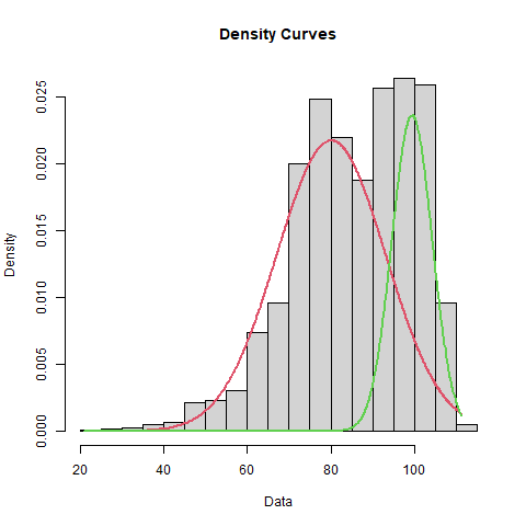
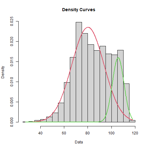
In our plots of distributions below, the red and green curves represent the two components of the mixed normal distribution that we fit for each player. Green represents the more well-struck contact and red represents more weakly contacted balls in play. The histograms are from the actual data and not from our parameterized distribution. Let's first look at Andrew McCutchen:

The histogram seems consistent with the hypothesis of a mixed normal distribution, and the green, solid contact portion of the mixture suggests that such well-struck balls have a mean of about 99.5MPH. Let's take a look at Mike Trout for comparison:

From the histogram, Trout's raw data doesn't exhibit the same two clear peaks as McCutchen's data. Their red curves (weak contact) are nearly identical though. The main difference is that Trout's green (solid contact) curve is about 6.2 MPH higher. This difference more than makes up for the fact that more of McCutchen's swings end up green.

Aside from insights we might gain from explorations like the above, one benefit of this parameterized distribution is that the parameters may be helpful in other, related analyses. For example, in my CASSIE projections, I may decide that I want to use exit velocity as part of my Bayesian prior for each player when projecting their offensive stats. The parameters that were fitted should be more informative than a simple average exit velocity parameter. However, we may decide to take one further step to simplify things. We may decide that the main piece of prior information we care about is the maximum velocity at which a player is capable of hitting the ball. Even mediocre batters can hit a few home runs over a short sample, but nobody flukes their way into hitting a ball 120MPH…a single instance of that represents demonstrable, informative skill. However, there is risk involved in overly focusing on a parameter, max EV, derived from only a single swing. We can mitigate this risk by using our parameterization of each player’s exit velocity distribution to give us a proxy for “max EV”. For instance, we may decide that the 99th percentile exit velocity from our newly parameterized distribution represents a good proxy maximum possible exit velocity for that player, so we can find that in the same R file from my public Github. The estimated max exit velocity for McCutchen came to about 111 to Trout's 115.

So to summarize, we recognized there are major problems with using the single parameter of mean exit velocity, but we see sometimes there are benefits to reducing a distribution to a single number. With the above approach, we were able to characterize a player’s exit velocity distribution by a single number while still recognizing the nonlinearity of exit velocity as it relates to the productivity of a batted ball. A primary use case for doing so is to act as part of a Bayesian prior in a projection model like my own CASSIE.